Loading
Classifying whether an image contains a dog or a cat is a classic computer vision challenge. Without computer vision techniques, solving this problem is nearly impossible. In this blog, we will walk through the process of designing an effective image classifier. Although there is no single architecture suitable for every type of image classification problem, some rules of thumb must be followed to create an effective image classification model.
Before diving in, make sure you have a basic understanding of:
For our example, we will be using the CIFAR-10 dataset, which consists of 60,000 (32x32) color images in 10 classes, with 6,000 images per class.
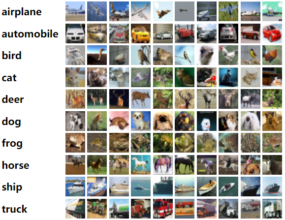
This dataset is pre-bundled with Keras, so if you are already using Keras and TensorFlow, you do not need to download it. Because we are working with images, having a GPU is helpful but not required.
Let's load the dataset and start coding.

The training and testing images are in a tuple format. If you print train_images[0], it will return a (32, 32, 3) tuple. This means the image has a height of 32 pixels, a width of 32 pixels, and 3 color channels (RGB). Each value in the array, ranging from 0 to 255, represents a pixel's intensity.
Here is where your image processing knowledge comes in handy. We know that in deep learning, a normalized pixel value (from 0 to 1) is more suitable. So, let's normalize them.
Now, if we print train_images[0], it will show us an array consisting of 32 arrays of 3-digit numbers ranging from 0 to 1 in decimal format.
We need to convert the integer labels of the images into one-hot encoded vectors because the neural network's output represents the probability that an image belongs to each class. In a one-hot encoding, if an image has a class label i, it is represented as a vector of length 10 (corresponding to the number of classes), where all elements are 0 except for the i-th position, which is set to 1.

We can easily one-hot encode our test_labels and train_labels using the to_categorical() function.
Now that we are done with our project setup, let's dive into the architecture. We will be using Keras's sequential architecture. You can also use the functional architecture, but there might be some syntactical differences.
If you have the prerequisite knowledge, you know what an MLP is. As a reminder, a multilayer perceptron, or MLP, is simply a neural network with multiple layers connected to each other. We will first build our model using only multilayer perceptrons.
As an example, we can create a simple MLP where:
Again, you need the prerequisite knowledge to fully understand the architecture.
So, the model will look something like this:
Now, if we plot the model summary using model.summary(), we will get an output similar to the following:

In the summary, you'll notice that the first value in the output shape is None. Keras uses None to indicate that the model can process any number of images simultaneously. Since the network performs tensor algebra, we don't need to pass images one by one; instead, we can process them in batches. For input images of shape (32, 32, 3), the input size is calculated as .
Now, let's examine the first dense layer. This layer contains 100 neurons, so the output shape is (None, 100). In the "Param" column of the summary, we see a value representing the total number of parameters (weights) trained at each layer. Here's how this number is computed:
Parameters = (input_size * output_size) + output_sizeSimilarly, we can calculate the parameters for the remaining dense layers:
dense_1 (50 neurons, input from dense layer): dense_2 (10 neurons, input from dense_1 layer): This formula accounts for both the weights (connections between neurons) and biases (one for each neuron). By following this method, we can determine the number of parameters for any dense layer in the model.
Now, let's train the model and evaluate its performance:
At this stage, I assume you are familiar with hyperparameters such as the loss function and optimizer. Since this is a multi-class classification problem, we use categorical_crossentropy as our loss function. For optimization, we use the default Adam optimizer, which is known for its adaptive learning rate and efficiency.
We train the model for 20 epochs with a batch size of 32:
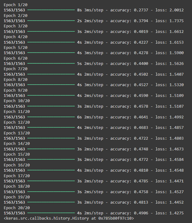
From the training results, we observe that the model achieves approximately 50% accuracy on the training dataset, which is relatively low. To further evaluate its performance, we test it on unseen data using model.evaluate(test_images, test_labels).
In my case, the model's accuracy on the test dataset is 46.96%, indicating potential overfitting or a suboptimal model architecture.
At this point, you can experiment with different architectures, hyperparameters, or preprocessing techniques to improve performance.
Convolution is another broad topic you need to understand to fully grasp why we are using a convolutional neural network. In short, convolution is a technique in which a small filter (called a kernel) slides across an input image, performing a dot product with each local region to extract features like edges or textures. By identifying patterns within the image, convolution essentially creates a new feature map.
In TensorFlow Keras, we use the Conv2D layer to apply convolutions to an input tensor:
Now, let's build a simple CNN model by adding a convolutional layer before a Multilayer Perceptron (MLP).
You can also check the model's summary by running cnn_model.summary(). Now let's compile and run the model.
After training, we evaluate the model on test data by running cnn_model.evaluate(test_images, test_labels), where the testing accuracy achieved is 59.11% (0.5911). This indicates an improvement, but we will continue refining our model in future experiments.
Testing accuracy is the key metric to measure how well our model generalizes to unseen data.
One other thing we can do is stack multiple CNN layers together. Let's add another CNN layer and see if the model improves.
Our model has improved, achieving an accuracy of 61.07%, but not significantly. Another important observation is that the training accuracy continues to increase, reaching almost perfect scores (98.27%). This indicates a problem: rather than learning meaningful features, the model is simply memorizing the training data, which means our model is overfitting.
To mitigate this problem, we can introduce a pooling layer.
The pooling layer in a CNN is used to reduce the spatial dimensions (width and height) of the input feature maps (the output of a conv layer, a matrix) while retaining important information. This helps in:
Now, let's explore the different types of pooling with a simple example.
Suppose we have a 4x4 matrix (feature map) after a convolution operation:
Now, let's apply different types of pooling.
In Max Pooling, we take the maximum value from each window (sub-region). Let's apply a 2x2 filter with a stride of 2 (moving 2 steps each time).
| Region | Max Value |
|---|---|
| (1, 2, 5, 6) | 6 |
| (3, 4, 7, 8) | 8 |
| (9, 10, 13, 14) | 14 |
| (11, 12, 15, 16) | 16 |
Why use Max Pooling?
Instead of taking the max value, Average Pooling takes the average of all values in each window.
| Region | Average Value |
|---|---|
| (1, 2, 5, 6) | 3.5 |
| (3, 4, 7, 8) | 5.5 |
| (9, 10, 13, 14) | 11.5 |
| (11, 12, 15, 16) | 13.5 |
Why use Average Pooling?
Instead of using a small window, Global Pooling applies pooling over the entire feature map.
Why use Global Pooling?
| Type of Pooling | Pros | Cons |
|---|---|---|
| Max Pooling | Keeps dominant features, reduces size | May lose less intense features |
| Average Pooling | Retains more information | Less emphasis on strong features |
| Global Pooling | Reduces feature maps to a single value | May lose spatial details |
Max pooling is the most commonly used in CNNs since it captures the most important features effectively.
In our case, let's add a MaxPooling layer and see what happens.
If we run the cnn_with_pooling model exactly as before, we find that the training accuracy has decreased to 0.9083, while the testing accuracy has increased to 0.6794 (your results may vary slightly). This is a positive outcome, as it suggests better generalization.
As there is room for improvement in training, increasing the total number of epochs could further improve the model's accuracy.
To further address the overfitting problem, we can also introduce a dropout layer. Dropout works by randomly disabling a fraction of neurons during training, preventing the network from relying too heavily on specific neurons. This encourages the model to learn more robust and generalized features.
In this model, we have introduced a Dropout(rate=0.3) which randomly disables 30% of the neurons after each convolutional layer. Running this model, we observe a reduction in training accuracy. In my case, after 20 epochs, the training accuracy was 0.7655, while the testing accuracy improved to 0.7211. This is great because both training and testing accuracy are increasing proportionally, indicating reduced overfitting. Additionally, running the model for more epochs may further improve the testing accuracy.
You can also apply dropout to the fully connected layers. Experimenting with different dropout rates and positions can help you understand how these changes affect model performance. Try adjusting these parameters and observe how the model behaves to find the optimal configuration.
We don't actually need a Batch Normalization layer for our example, but it's still worth exploring because it plays a crucial role when working with large datasets.
Batch Normalization (BN) is a technique used in deep learning to make training faster and more stable. It does this by normalizing the outputs of each layer, ensuring they have a steady distribution. This helps in:
In deep learning, when the network updates its weights, the distribution of inputs to each layer can change. This makes training slow and unstable. Batch Normalization helps by keeping the data in a fixed range so the network can learn efficiently.
Think of it like a classroom: If a teacher changes the grading scale every week, students would struggle to understand their progress. But if the scale stays the same, it's easier to track improvements. BN ensures the "grading scale" for data remains stable throughout training.
Although we don't need batch normalization in our example, let's still implement it.
Let's say we have a small batch of numbers:
To make the values easier to process, we subtract the mean and divide by the standard deviation:
For example:
Now, the values are adjusted to be around 0, which helps learning!
Batch Normalization introduces two parameters: gamma () and beta (), which adjust the data after normalization:
This allows the model to adjust values to the best scale and shift for learning.
BN is usually applied before or after activation functions. The typical order is:
| Advantage | Why It's Useful |
|---|---|
| Faster Training | Reduces the need for careful weight initialization, speeding up learning. |
| More Stable Training | Keeps the network's activations in a consistent range. |
| Better Generalization | Acts like regularization and prevents overfitting. |
| Less Reliance on Dropout | Can reduce the need for dropout to prevent overfitting. |
Batch Normalization helps neural networks learn faster, more reliably, and with better generalization. By normalizing data within mini-batches, it ensures stable activations and reduces internal covariate shift.
As mentioned earlier, we don't need Batch Normalization in our example. If you run the model with Batch Normalization, you'll notice little to no change in training and testing accuracy. However, for demonstration purposes, I have added both the BatchNormalization() and Dropout() layers to show that we can also modify the fully connected layers. This highlights how these layers can be incorporated into different parts of the network to potentially improve performance.
The provided architecture is not the most efficient, and there are several ways to optimize it. For example, the number of filters in each Conv2D block should be tailored to the specific task. To keep this example simple, I have used the same number of filters for all Conv2D layers, but in practice, adjusting the filters can improve performance. Similarly, there are many other ways to design a model based on your specific needs, such as adjusting layer configurations, adding skip connections, or experimenting with different activation functions.
There is no exact formula for building an image classification model or any AI model for that matter. Achieving a robust and high-performing model requires experimenting with different architectures and tuning hyperparameters to find the best configuration for your specific dataset.
In this blog, we explored various fundamental layers used in deep learning:
layers.Dense(...) – The standard dense layer used for classification and feature learning.layers.Flatten() – Converts multi-dimensional feature maps into a 1D vector for the fully connected layers.layers.Conv2D(...) – Extracts spatial features from images by applying learnable filters.layers.MaxPooling2D(...) – Reduces spatial dimensions and computational complexity while retaining important features.layers.Dropout(...) – Prevents overfitting by randomly deactivating a fraction of neurons during training.layers.BatchNormalization() – Normalizes activations to stabilize training and improve convergence.Each of these layers has variations that can be used to improve model performance:
Conv1D(...) – Used for sequential data like time-series or text.Conv3D(...) – Used for 3D image data, such as medical imaging.SeparableConv2D(...) – A depthwise-separable convolution that reduces computational cost.AveragePooling2D(...) – Computes the average of a region instead of the max value, useful for certain tasks.GlobalMaxPooling2D(...) – Reduces the entire feature map to a single value per filter, useful before fully connected layers.Dropout(0.5)) prevent overfitting, while lower values (e.g., Dropout(0.1)) provide mild regularization.Using these foundational layers, we can construct more advanced architectures:
Conv2D, BatchNormalization, ReLU, and an Add layer to enable skip connections. This technique helps in training deep networks by mitigating the vanishing gradient problem.Dense and Pooling layers along with matrix operations, which focus on important regions in an image. This concept is widely used in Vision Transformers (ViTs) and Attention Mechanisms.By combining these techniques, you can design more efficient and powerful deep learning models tailored to your specific problem. Experimenting with different architectures and hyperparameters will help you find the best approach for your dataset.

